Principle and design of power control and calibration for CDMA mobile station
In order to ensure that the radio frequency index of each CDMA mobile station meets the requirements of the industry standard (3GPP2) and the performance of the CDMA network, it is necessary to perform radio frequency calibration on each mobile station. Before discussing the RF calibration algorithm, the principle of the CDMA mobile station power control algorithm is first explained. There are a large number of analog devices in the radio frequency circuit of the CDMA mobile station, and the analog devices have great device dispersion.
RASRAM linear control principle
The baseband mobile station power control algorithm uses the RASRAM linear control principle. Because the linearity of the intermediate frequency (IF) AGC amplifier is not good, the amount of gain attenuation is not proportional to the magnitude of the gain control voltage. In other words, the change in attenuation is not proportional to the change in control voltage, and the function of attenuation and gain control voltage is non-linear. The RAS (Rf Analog System) RAM linearizer generates a variable gain amplification control voltage, so that the Pulse Density ModulaTIon (hereinafter referred to as PDM) drive circuit compensates for the aforementioned nonlinear characteristics. RAS RAM linearizer is a simple conversion function. It uses a programmable piecewise linear function to linearize the RAS RAM linearizer input and attenuation after calibration.
CDMA mobile station RF calibration algorithm
The power calibration part of the reference channel (reference channel for power control) is the most basic and important part of the entire CDMA mobile station calibration system, and its accuracy is related to the power accuracy of the entire system. Among various power calibration algorithms, there are two main algorithms commonly used in the industry: iterative power measurement algorithm and linear fitting algorithm. The principles of these two algorithms and the implementation process in CDMA mobile station power calibration are introduced below.
1 Basic algorithm of linear fitting
The linear fitting algorithm is divided into two algorithms: optimal difference compensation and extension, and the calculation mathematical models of the two algorithms are the same. The following uses the optimal difference compensation algorithm as an example to introduce.
Assume that the ideal output power array of the mobile station is:
Table [i] =-66.8; -63.6; -60.4; -57.2; -54; -50.8; -47.6; -44.4; -41.2; -38; -34.8; -31.6; -28.4; -25.2; -22; -18.8; -15.6; -12.4; -9.2; -6; -2.8; 0.4; 3.6; 6.8; 10; 13.2; 16.4; 18; 19.6; 21.2; 22.8; 24.4; 26; 27.6;
29.2; 30.8; 32.4; 34; 35.6; 37.2; 38.8; 40.4; 42; 45.2; 48.4; unit: dBm.
For each ideal output power test point, after the ideal output power Table [i] is determined, the PDM compensation value can be obtained by interpolation from other nearest neighboring power test points.
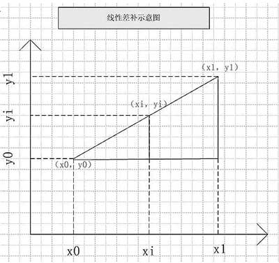
Figure 1 Linear difference compensation method
As can be seen from Figure 1,
Yi-y0 = K (xi-x0) = (y1-y0) / (x1-x0) * (xi-x0) (1)
Move y0 to the right,
Yi = K (xi-x0) = (y1-y0) / (x1-x0) * (xi-x0) + y0 (2)
It is known that Yi = Table [i], y1 and y0 are the nearest neighbor test power values, x0 and x1 are the PDM values ​​corresponding to the test power of the nearest neighbor test points, and xi is the corresponding PDM value of the desired ideal output power.
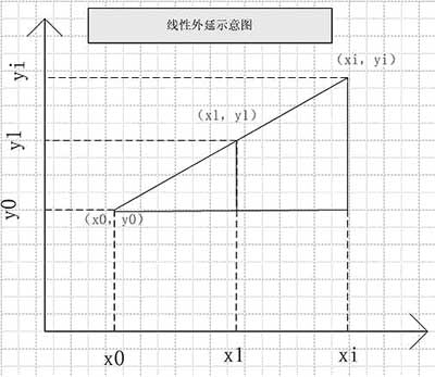
Figure 2 Linear epitaxy
If the desired ideal output power level falls outside the range of the test power level, then it needs to be calculated by the epitaxy method as shown in Figure 2, the principle is the same as above, and will not be repeated.
2 Linear fitting process
First, the CDMA output power level is divided into two groups: high power level and low power level. In each group, it is divided into several test points according to the dynamic range of power control. During the test, each point is tested to obtain the corresponding power control pin voltage (corresponding to the PDM value) and the power amplifier output power value, and then through the linear The fitting results in an approximately linear relationship between the voltage of the power control pin at this power level and the output power of the power amplifier.
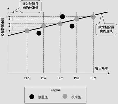
Figure 3 A calibration algorithm used in actual production
Finally, the voltage value of the corresponding power control pin is calculated according to the ideal output power required by different power levels in the power level group.
This calibration process needs to be performed on the two high and low power levels. Up to 64 points can be tested at most. After the above calibration, the accuracy of the CDMA mobile station's transmit power can reach about ± 0.4dB.
3 Linear fitting characteristics
Advantages: each power point calibration is only measured once, the calibration speed is fast, the production cycle is fast, and the production cost is low.
Disadvantages: If the measured power value does not fall within the range of the optimal difference compensation, due to the simulation of the cathode characteristics of the RF hardware, the power voltage curve is nonlinear, but the program algorithm will be calculated according to the linear epitaxy algorithm, resulting in the calculated value The power value has a large accuracy gap, and the test accuracy is low.
4 Basic algorithm for iterative power measurement
The characteristic curve of mobile station power voltage can be regarded as a nonlinear function. The power voltage characteristic curve of a nonlinear function can be fitted by dividing the curve into 36 small segments, and each segment can be regarded as a function of a linear relationship.
According to the characteristics of different power curve segments, in order to improve the convergence speed and increase the concept of the convergence factor K, the above CDMA power iterative measurement formula is converted into a piecewise iterative formula, and the parameters are instantiated as follows:
X1 (n + 1) -X1 (n) = (int) 4 * (Y1 (n) -Ynd) The initial value Xd is the physical characteristic as the driving voltage value. Xd [36] = {100,120,140,170, ... 460,480} Ynd is the ideal output power. Ynd [36] = {48.4, 45.2; 42, 38.8, 35.6, 32.4, 29.2, 26, 22.8, 19.6, 16.4, 13.2, 10, 6.8, 3.6, 0.4, Among them, the unit is dBm, the convergence factor K = 3, 4, 5, 6. Iterative algorithm is a basic method for solving problems with computer. It takes advantage of the computer's fast computing speed and suitable for repetitive operations, allowing the computer to repeatedly execute a group of instructions (or certain steps), and each time the group of instructions (or these steps) is executed, the original value of the variable is used. Launch a new value for it. However, to solve the problem using an iterative algorithm, the following three steps are required. Determine iteration variables. Among the problems that can be solved by iterative algorithms, there is at least one variable that directly or indirectly continuously pushes the new value from the old value. This variable is the iterative variable. Establish an iterative relationship. The so-called iterative relationship refers to how to derive the formula (or relationship) of the next value from the previous value of the variable. The establishment of the iterative relationship is the key to solving the iterative problem, and it can usually be done by using recursive or backward methods. Control the iterative process. When does the iteration process end? This is an issue that must be considered when writing an iterative program. The iteration process cannot be repeated endlessly. The control of the iterative process can usually be divided into two cases: one is that the required number of iterations is a certain value and can be calculated; the other is that the required number of iterations cannot be determined. For the former case, a fixed number of loops can be constructed to control the iterative process; for the latter case, the conditions used to end the iterative process need to be further analyzed. For the algorithm to realize the power correction function of the mobile station, which belongs to the latter case, the iterative suspension rule usually adopts fabs (Y (n) -Yd) <ε (where ε> 0 is the set relative error tolerance) . Here, according to the system error of the test system, we take ε = 0.2dB. According to the circuit driving principle of PA, in a certain characteristic curve, the output power can be regarded as a linear relationship of K times the PA input voltage, so there can be △ x = K △ y + θ, that is: X (i + 1) -X (i) = K (Y (i) -Y (d)) + θ, θ is a fixed constant. We can use this as an iterative formula and use the computer to find the exact voltage value corresponding to a certain power (under the premise of a certain iteration accuracy ε). The single point power three iteration process is shown in Figure 4. Figure 4 Iterative algorithm principle Obviously, the number of single-point iterations is greatly affected by the convergence factor K. The larger the K, the fewer the iterations, but the lower the iteration accuracy; conversely, the smaller the K, the more iterations, but the higher the iteration accuracy. According to the above analysis, for each power point, the CDMA power iterative measurement formula can be described in mathematical language as follows: X (n + 1) -X (n) = (int) K * (Y (n) -Yd) K is the convergence factor, Y (n) is measured by the measuring instrument when the mobile station sends the X (n) PDM value; Yd is the ideal output power when the mobile station power voltage curve is linear. Initial condition: X (0) = Xd Xd is the initial value of the mobile station's iterative PDM transmission. 5 Power iterative measurement implementation process The CDMA output power level is divided into two groups: high power level and low power level. In each group, it is divided into several test points according to the dynamic range of power control. During the test, firstly according to the ideal output power required by the different power test points selected in the power level group, a power iterative measurement algorithm is used to gradually send the PDM, and the emitted power value is measured until the ideal output power is reached, then the The obtained PDM is written into the calculation linked list. According to the calculation list, combined with the ideal output power required by the different power levels that have not been selected, the correspondence calculation list between the voltage of the power control pin at that power level and the ideal output power of the power amplifier is obtained through interpolation and extension. In order to meet the power control accuracy requirements of CDMA mobile stations. This calibration process needs to be performed on the two high and low power levels. After the above calibration, the accuracy of the CDMA mobile station's transmission power can be controlled within the test error range of the system. 6 Power iterative measurement characteristics Features: slow calibration speed, high production cost and high accuracy. Advantages: Because the error between the measured value and the ideal output power can be controlled by adjusting the relative error tolerance, the test accuracy can be controlled relatively high (in the best case, it is controlled within the system error of the test system), and can also be controlled Relatively low. Disadvantages: Because the selected iteration factor K is different for each power point measurement, the number of iterations is more or less, and at least one power measurement is performed at each point, so the calibration speed is slow, the production cycle is slow, and it will occupy more valuable production Instrument test resources, so production costs are relatively high. Conclusion In summary, the power iterative measurement algorithm and the linear fitting algorithm each have advantages and disadvantages. Given that the power control accuracy of the CDMA system controls the power change accuracy of the mobile station in steps of 1 dB, and at the same time considers the production cost of mobile station test calibration, combined with the linear fitting algorithm is fast, and the calibration accuracy also meets the system requirements, In the research and development engineering practice, the linear fitting algorithm is generally selected to realize the production power correction algorithm of the CDMA mobile station. The Rockwell Controllogix processor provides an optional user Memory Module (750K to 8M bytes) that can solve application problems with a large number of input and output points systems (up to 4000 analog and 128000 digital bits). The processor can control local input and output and remote input and output. The processor can monitor input and output in the system via Ethernet EtherNet / IP, ControlNet ControlNet, DeviceNet DeviceNet, and Remote I/O Universal Remote I / O.
The ControlLogix system is a rack-mounted, modular installation. The Controllogix I/O Modules are modularly mounted. The power module is mounted directly to the left side of the ControlLogix chassis. The Controllogix chassis is available in five types of 4, 7, 10, 13 or 17 slots. The module can be inserted in any slot of the rack. The maximum number of channels for Controllogix I/O modules is 32 channels. The mechanical lock of the removable terminal block of each module prevents the application of erroneous voltages to the module. Input and output modules can be hot plugged.
Rockwell Allen-Bradley: SLC500/1747/1746 MicroLogix/1761/1763/1762/1766/1764
(Y1 (n) -Y1d) <4, Y1 (n) <17dbm, 0
(Y2 (n) -Y2d)> = 4, Y2 (n) <17dbm, 0
(Y3 (n) -Y3d) <3, Y3 (n)> = 17dbm, 0
(Y4 (n) -Y4d)> = 3, Y4 (n)> = 17dbm, 0
-2.8, -6, -9.2, -12.4, -15.6, -18.8, -22, -25.2, -28.4, -31.6, -34.8, -38, -41.2, -44.4, -47.6, -50.8, -54 , -57.2, -60.4} 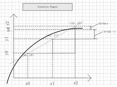
The first iteration: X0 = Xd, Y0-Yd> ε, does not satisfy | Y0-Yd | <ε iteration stop condition, continue to iterate;
The second iteration: X1 = X0, Y1-Yd> ε, which does not satisfy | Y0-Yd | <ε iteration stop condition, continue iteration;
The third iteration: X2 = X1, Y2-Yd <ε, satisfying | Y0-Yd | <ε iteration stop condition, stop iteration; X2 is the required PA input voltage value (iteration accuracy ε precondition: ε = 0.2 dB). 
When there are multiple processor modules in the Controllogix chassis, and even if there are multiple processor modules in the ControlNet network of the control network, all processors can read input values from all input modules. Any one processor can also control any specific output module. The system configuration specifies which processor is controlled by each output module.
CompactLogix/1769/1768
Logix5000/1756/1789/1794/1760/1788,PLC-5/1771/1785 and so on.

Rockwell Allen-Bradley
Rockwell Allen-Bradley,Processor Controll,Rockwell Automation Allen-Bradley,Allen-Bradley Equipments
Xiamen The Anaswers Trade Co,.LTD , https://www.answersplc.com