
"In some respects, machine vision is better than human vision. But now researchers have found a class of 'antagonistic images' that can easily 'fool' machine vision." - Emerging Technology from arXiv.
One of the greatest advances in modern science is the rise of machine vision. In recent years, a new generation of machine learning technology has changed the way that computers "see" the world.
Machines now surpass humans in face recognition and item identification, and will change countless vision-based tasks such as driving, security monitoring, and more. Machine vision is now Superman.
But there is a problem. Machine vision researchers have noticed that this new technology has some worrying weaknesses. In fact, machine vision algorithms have an Achilles heel that makes them tricky by some perturbed images that are very easy to see for humans.
These modified images are called "antagonistic images and become an important threat." In the field of face recognition, a confrontational example may consist of very subtle marks on the face, so people will correctly recognize the image. Identity, and the machine learning system will identify it as a different person. "Google Brain's Alexey Kurakin, Samy Bengio and Ian Goodfellow of the nonprofit OpenAI said.
In their paper, they stated that this adversarial attack can affect systems that run entirely on computers, such as escaping spam filters or virus software monitors, but can also affect systems that operate in the physical world, such as through cameras and other Sensors perceive the world's robots, video surveillance systems, and mobile applications for image and sound classification.
Because machine vision is still very new, we know little about adversarial images. No one knows how to best create them, how to use them to fool the machine vision system, or how to prevent such attacks.
Now, Kurakin and colleagues' research has begun to change this situation. They have systematically studied antagonistic images for the first time. Their research illustrates how fragile the machine vision system is under such attacks.
The team began using a standard database for machine vision research called ImageNet. The image of this database is categorized according to the displayed content. A standard test is based on a part of this database to train a machine vision algorithm, and then use another part of the database to test whether the algorithm can be well classified.
The test performance is measured by the frequency of the top five answers in the statistical algorithm, and even the correct classification in the highest one (referred to as the first five accuracy and the previous accuracy rate), or the answer in the top five or one item is not The correct frequency (the first five error rates or the previous error rate).
One of the best machine vision systems is Google's Inception v3 algorithm, and its top five error rate is 3.46%. The top five error rate for humans performing the same task is about 5%, so Inception v3 does have superhuman capabilities.
Kurakin and colleagues modified 50,000 ImageNet images in three different ways, creating a database of confrontational images. Their approach is based on the concept that neural networks process information to match an image to a category. The amount of information required for this process is called cross-entropy, which reflects the difficulty of matching tasks.
Their first algorithm makes a small change to the image in an attempt to maximize this cross-entropy. Their second algorithm simply iterates this process and further changes the image.
Both algorithms have changed the image, making it more difficult to classify correctly. "These methods can lead to some boring misclassifications, such as mistaking a sled dog for another sled dog."
Their final algorithm has a smarter approach. This change to the image gives the machine vision system a certain classification error and tends to be the most unlikely category. "The most unlikely classification is usually very different from the correct classification, so this method will cause more interesting mistakes, such as mistake a dog as an aircraft." Kurakin and colleagues said.
Then they tested whether the Google Inception v3 algorithm could well classify 50,000 adversarial images.
These two simple algorithms greatly reduce the first five and the previous accuracy. But their most powerful algorithm, the most unlikely taxonomy, quickly reduced the accuracy of all 50,000 images to zero. (The team did not disclose whether the algorithm was successful in guiding misclassification.)
This means that confrontational images are an important threat, but this method also has a potential weakness. All confrontational images are directly input into the machine vision system.
But in the real world, the image always changes through the camera system. If this process neutralizes its effect, an antagonistic image algorithm is useless. Therefore, it is important to understand how the algorithm responds to real-world changes.
For the test, Kurakin and his colleagues stated that all confrontational images and original images were printed and manually photographed with a Nexus 5 smartphone. Then, these transformed and confrontational images are input into the machine vision system.
Kurakin and colleagues say that the most unlikely category approach is the most affected by these shifts, but the tolerance of other approaches is fine. In other words, confrontational image algorithms are indeed a threat in the real world. "A lot of the confrontational images made with the original network were misclassified, even though the classifier was entered via the camera," the team said.
This study is very interesting and brings new insights into the vision of Achilles on machine vision. And there is still much research to do in the future. Kurakin and colleagues hope to develop confrontational images for other types of vision systems to make them more efficient.
This will lead to discussions in the field of computer security. Machine vision systems are now able to recognize human faces more than humans, so it's natural that we think of using this technology in more fields, from unlocking smartphones and homes, to passport control, and to bank account identities. But Kurakin and his colleagues proposed the possibility of easily "fooling" these systems.
In recent years, we have often heard how good a machine vision system can be. Now we have discovered that they still have stupid Achilles' heels.
Here, Lei Feng network (search "Lei Feng network" public number attention) for everyone to share from Google Brain and OpenAI scientists, entitled "The Antagonist in the physical world" full paper.
Summary
Most of the existing machine learning classifiers are easily affected by the examples of confrontation. A case of confrontation is an input data sample that has undergone some kind of perturbation in order to make the machine learning classifier misclassify. In many cases, these perturbations are so tiny that human observers may not notice these changes at all, and classifiers still make mistakes. Antagonistic examples raise security concerns because they can be used to attack machine learning systems, even if confrontation does not involve the underlying model. So far, all previous studies have assumed a threat model in which confrontation performance inputs data directly into the machine learning classifier. However, this is not always the case for systems operating in the physical world, such as those systems that use signals from cameras or other sensors as input. This paper shows that even in such a physical world scenario, machine learning systems can be affected by examples of confrontation. We demonstrate this by importing an image of the confrontation obtained from the camera of the phone into an ImageNet Inception classifier and measuring the classification accuracy of the system. We have found that a large proportion of confrontational examples are misclassified, even for images obtained from cameras.
1 Introduction
Recent advances in machine learning and deep neural networks allow researchers to address several important practical issues such as imagery, video, text classification, and others (Krizhevsky et al., 2012; Hinton et al., 2012; Bahdanau et al. , 2015).
However, machine learning models are often affected by the adversarial operations in their system inputs in order to trigger misclassification (Dalvi et al., 2004). In particular, many other categories, such as neural networks in machine learning models, are particularly vulnerable to attacks based on small modifications in system input at the time of testing (Biggio et al., 2013; Szegedy et al., 2014; Goodfellow et al., 2014. Papernot et al., 2016b).
The problem can be summarized as follows. Assuming there is a machine learning system M and input sample C, we call it a clean example. Assume that the correct classification in the machine learning system in Sample C is: M(C) = ytrue. We can create a confrontational example A that is indistinguishable from C but is misclassified systematically, namely: M(A) ≠ytrue. These adversarial examples are misclassified more frequently than examples that change by noise, even if the breadth of the noise exceeds the breadth of the adversarial effects (Szegedy et al., 2014).
The adversarial example poses a potential security threat to practical machine learning applications. Among them, Szegedy et al. (2014) proposed an adversarial example specifically designed to be misclassified in model M1, which is often misclassified by model M2. The transferable nature of this adversarial example means that we can generate adversarial examples, and we can misclassify machine learning systems without involving the underlying model. Papernot et al. (2016a,b) proved this type of attack in real-life situations.
However, all previous research on adversarial examples for neural networks utilized a threat model in which an attacker provided input directly into a machine learning model. In this way, adversarial attacks rely on good debugging of input data modifications.
Such a threat model can describe scenarios in which the attack occurs entirely in the computer, for example as an escape spam filter or virus software monitoring (Biggio et al., 2013; Nelson et al.). However, in practice many machine learning systems operate in a physical environment. Possible examples include, but are not limited to, robots that sense the world through cameras and other sensors, video surveillance systems, and mobile applications for image and sound classification. In such situations, confrontation cannot rely on good pixel-based adjustments in the input data. This raises the question of whether it is possible to create adversarial examples, conduct adversarial attacks on machine learning systems operating in the physical world, and perceive data through various sensors rather than digital representations.
Some previous research has explored the physical attack problem of machine learning systems, but it does not fool neural networks by creating tiny disturbances in the input. For example, Carlini et al. (2016) show that an attack creates a voice input that the mobile phone recognizes as containing meaningful voice commands, whereas humans sounds like meaningless words. Photo-based face recognition systems are vulnerable to replay attacks, in which the camera is presented with an image of the face that was previously authorized by the authorized user, rather than an actual face (Smith et al., 2015). In principle, adversarial examples can be applied to any one of the physical domains. A case of confrontation in the field of speech commands would include a recording (eg, a song) that looks harmless to humans, but contains the voice instructions that the machine learning algorithm will recognize. An example of confrontation in the field of facial recognition may include very subtle changes in the face, so a human observer will correctly identify their identity, but the machine learning system will recognize them as a different person.
In this paper, we explore the possibility of creating confrontational examples for image classification tasks in the physical world. For this purpose, we performed an experiment with a pre-trained ImageNet Inception classifier (Szegedy et al., 2015). We generated examples of confrontation for this model, and then used these examples to input classifiers through a cell phone camera and measure the classification accuracy. This scenario is a simple physical world system that senses data through a camera and then runs an image classifier. We have found that a large proportion of adversarial examples generated from the original model are still misclassified even though they are perceived by the camera.
Surprisingly, our attack method does not need to make any changes to the appearance of the camera - this is the use of confrontational examples, the simplest attack for the Inception model, it brings the success of the adversarial example transferred to the camera and Inception The combination of models. Therefore, our results give a lower attack success rate that can be achieved through more targeted attacks, and the camera is obviously simulated when building a case of confrontation.
The limitation of our results is that we assume a threat model where the attacker fully understands the model architecture and parameter values. This is basically because we can use a single Inception v3 model in all experiments without the need to set up and train different efficient models. The transitory nature of the antagonistic example means that when the attacker does not understand the model description, our results may be weakly extended into the scenario (Szegedy et al., 2014; Goodfellow et al., 2014; Papernot et al., 2016b. ).
To better understand how important image transitions caused by cameras affect the metastasis of counter-resistance examples, we conducted a series of additional experiments to investigate how the adversarial examples were transferred in several specific types of image transformation synthesis.
The rest of the paper will be organized as follows: In Part 2, we review the different methods used to generate examples of confrontation. The next section will discuss our "physical world" experimental setup and results in detail. Finally, Section 4 describes experiments using various artificial image transformations (such as changing brightness, contrast, etc.) and how they influence the example of confrontation.
2, the method of generating an antagonistic image
This section describes the different methods of generating an antagonistic image that we use in our experiments. It is worth noting that none of the described methods guarantees that the generated image will be misclassified. However, we call all generated images "antagonistic images."
In the rest of the paper we will use the following tags:
X - An image, usually a 3D tensor (length x width x height). In this paper, we assume that the pixel value is an integer between [0,255].
Ytrue - The real category of image X.
J(X,y) - Cross-entropy cost function of neural network based on image X and category y. We intentionally neglect neural network weights (and other parameters) θ in the cost function because we assume that they are fixed in the conditions of the paper (fixed to the value of the training machine learning model). For a neural network with a softmax output layer, the cross-entropy cost function applied to an integer-type label is equal to the negative logarithm probability of the real class: J (X, y) = - log p (y | X). Used below.
Clip X, ∈ {X' } - Runs a pixel-by-pixel clip of the image X', so the result will be around L∞ ε - around the original image X. The detailed clipping equation is as follows:

Where X (x, y, z) is the z-axis value of image X at coordinates (x, y).
2.1 Quick method
One of the easiest ways to generate confrontational images is as described by Goodfellow et al. (2014). The goal is to linearize the cost function and to solve the cost of maximizing L∞ constraints. This can be closed to achieve, only need to call back propagation once:

Where ε is a hyperparameter to be selected.
In this paper, we call this method a "fast method" because it does not require an iterative process to calculate adversarial examples, which is faster than other methods considered.
2.2 Basic Iteration Method
We have introduced a straightforward way to extend the "fast" method - we apply it multiple times in small steps, and cut the pixel values ​​of the intermediate results after each step to ensure that they are in the perimeter of the original image. Inside:

In our experiment, we use α = 1, that is, we change the value of each pixel by only one at each step. We choose the minimum number of iterations (ε + 4,1.25 ε). This number of iterations is chosen in a heuristic way; this is enough to make the adversarial case reach the maximum norm of ε, while there are enough limits to allow the experimental calculation cost to be within the control range.
We will call this method the "basic iteration" method below.
2.3 Iteration Most Impossible Category Method
The two methods that we have described so far are simply trying to increase the cost of the correct type, but not which type of model the model should choose. Such an approach is sufficient for database applications, such as MNIST and CIFAR-10, where the number of types is small and the types vary widely. In ImageNet, the number of types is much larger, and the differences between different categories are different. These methods may cause more boring misclassifications, such as mistake a sled dog as another sled dog. In order to create more interesting misclassifications, we introduced the iterative most unlikely class approach. The confrontational images that this iterative method attempts to make will be classified as a specific target category based on expectations. As for the desired category, we use neural networks trained based on image X training to predict and select the most unlikely category:

For a well-trained classifier, the most unlikely class is usually highly different from the real class, so this attack method creates more interesting errors, such as misidentifying a dog as an airplane.
To make an antagonistic image classified as yLL, we proceed to iterative steps in that direction: 
Maximize log p(yll | X). The last equation is equivalent to a neural network with cross-entropy loss:  .
.
In this way, we have the following steps:

For this iterative process, we use the same alpha and the same number of iterations as the basic iterative method.
Below we call this method the "Most Impossible Class" method, or "ll Class" for short.
2.4 Comparison of methods for generating antagonistic examples
As mentioned above, confrontational images are not guaranteed to be misclassified - sometimes attackers win, and sometimes machine learning models win. We have done experimental comparisons of antagonistic methods to understand the actual classification accuracy of the generated images and the type of perturbation used by each method.
The experiment used a total of 50,000 verification images from the ImageNet database (Rusakovsky et al., 2014) using a pre-trained Inception 3 classifier (Szegedy et al., 2015). For each verification image, we use different methods and different ε values. For each set of methods and ε, we calculate the classification accuracy on all 50,000 images. In addition, we calculate the accuracy on all clean images and use them as benchmarks.
Examples of generated antagonistic images are shown in Figures 1 and 2. The first and first five classification accuracy for clean images and confrontation images are summarized in Figure 3.
As shown in Table 3, even if the fast method uses the minimum value of ε, it also reduces the former precision by one half, and reduces the first five precision by about 40%. As we increase the ε value, the fast method generates The accuracy of the confrontational image remains constant until ε = 32, then slowly decreases to approximately 0 as ε increases to 128. This can be explained by the fact that the fast method increases the noise of ε times for each image, so a higher ε value actually destroys the image content, even if it is not recognized by humans (see Figure 1).
The iterative method uses many better perturbations, even if the higher ε value does not destroy the image, see Figure 2.
The basic iterative method can generate a better confrontational image when ε < 48, but it cannot be improved when we increase the ε value.
The "Most Improbable" method destroys the correct classification of most images even when ε is relatively small.
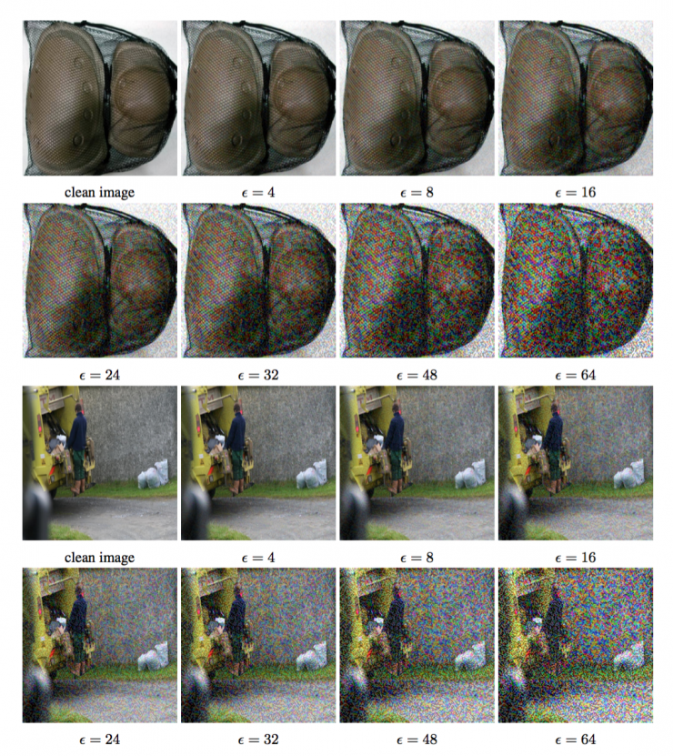
Figure 1: Comparing images that resist fast perturbations using the "fast" method. The top image is a "knee pad" and the bottom image is a "garbage truck." In both cases, the clean images were correctly classified, and the antagonistic images were misclassified in all the considered ε values.
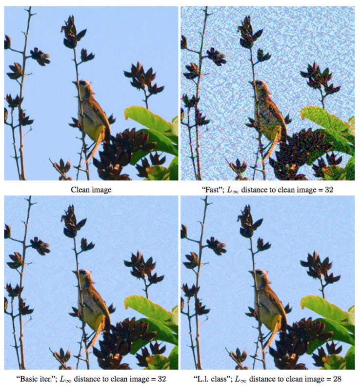
Figure 2: Using ε = 32, compare different methods of confrontation. The perturbation generated by the iterative method is better than the fast method. In addition, the iterative method does not always select the point on the ε-peripheral boundary as an antagonistic image.

Figure 3: The first and fifth precision of Inception v3, and the different ε values ​​compared to the "clean image" - unmodified image in the database, under the attack of the non-antagonistic method. Accuracy is calculated using a total of 50,000 verification images in the ImageNet database. In these experiments, the ε value ranged from 2 to 128.
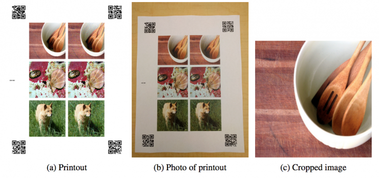
Figure 4: Experiment setup: (a) Generated prints, containing clean images and an antagonistic image group, and a QR code to help auto-cut; (b) Photo prints made by a cell phone camera; (c) Automatically from photos Cut image.
We further limit all subsequent experiments to ε ≤ 16, because even if such fine tuning is recognized, it is only considered as a small noise, and the antagonistic method can generate enough within the ε-periphery of the clean image. Examples of misclassification of quantities.
3. Image of an adversarial example
3.1 Destruction rate of confrontational images
In order to study the impact of coercive transformation of confrontational images, we introduced the concept of destruction rate. It can be described as the proportion of the confrontation images that can no longer be misclassified after conversion. The formulation is defined as equation (1) below:
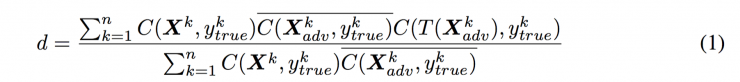
Where n is the number of images used to calculate the destruction rate and X k is an image in a database.  Is the real category of this image,
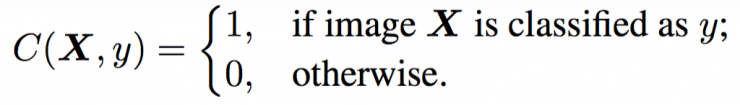
  It is a corresponding confrontational image. The function T() is a mandatory image transformation. In this paper, we study various transformations, including printing images and taking pictures of the results. The function C(X, y) is an indicator function and the returned image is correctly classified:
We mark the binary negative of this indicator value as  The calculation method is
  = 1 - C (X, y ).
3.2 Experiment Settings
To explore the possibility of physical confrontational examples, we performed a series of experiments using pictures of antagonistic examples. We printed a clean picture and an antagonistic picture, took a picture of the printed page and cut out the printed picture from the full page. We can think of this as a black box transformation. We call it "photo conversion."
We used clean images and confrontational images to calculate the accuracy before and after the photo conversion, and calculate the destruction rate of the image due to the conversion of the photos.
The experimental process is as follows:
1, print the image, as shown in Figure 4a. In order to reduce manual work, we printed multiple sets of clean and antagonistic examples on each sheet. In addition, two-dimensional codes are placed on the printed corners to help with automatic cutting.
All printed generated images (Figure 4a) are saved in lossless PNG format.
Batch PNG printing uses the default setting in the ImageMagick package: convert .png output.pdf to convert to a multi-page PDF document.
The resulting PDF document is printed using a Ricoh MP C5503 office printer. Each page of the PDF document is automatically resized using the default printer resizing to fit the entire sheet. The printer pixel is set to 600 dpi.
2. Use a mobile phone (Nexus 5x) to take a picture of the printed image, see Figure 4b.
3. Automatically cut and wrap the validation examples in the image so that they will become the same size square as the original image, see Figure 4c:
(a) Monitor the position and value of the four two-dimensional codes on the four corners of the photo. The QR code contains the batch information of the verification example shown in the picture. If you do not successfully monitor any corners, the entire image will be abandoned and the images in the photos will not be used to calculate accuracy. We observed that no more than 10% of all images in any experiment were discarded, and images that were usually discarded were approximately 3% to 6%.
(b) Use perspective transformations to wrap the image so that the position of the two-dimensional code is moved into predefined coordinates.
(c) After the image is wrapped, each of the examples has known coordinates that can be easily cut out of the image.
4. Run the classification on the converted image and the original image. Calculate the accuracy and destruction rate of the confrontation image.
This process involves manually photographing the printed pages without having to carefully control factors such as lighting, camera angle, and distance to the page. This is intentional; this introduces subtle changes that can destroy adversarial perturbations because it relies on subtle, well-adapted, accurate pixel values. However, we did not intentionally use extreme camera angles or lighting conditions. All photos were taken in normal indoor lighting, with cameras facing the page in general.
For each group of antagonistic example generation methods and ε, we performed two sets of experiments:
Average situation:
To measure the average performance, we randomly selected 102 images in one experiment, using an established ε and antagonistic method. This experiment estimates the frequency with which a successful attack chooses to randomly select photos - the outside world randomly selects an image, and confrontation attempts to misclassify it.
Pre-screening situation:
In order to study more aggressive attacks, we experimented with pre-screened images. Specifically, we selected 102 images so that all clean images were correctly classified, and all confrontational images (before the images were converted) were misclassified (both the first and the first five categories). In addition, we use a confidence threshold for the highest prediction: p (yyyyyyyyy) ≥ 0.8, where ypredicted is the category of image X predicted by the network. This test measures the frequency of success when confrontation can choose which of the original images to attack. Under our threat model, confrontation can involve the parameters and architecture of the model, so attackers can always intervene to determine whether the attack will succeed if there is no photo conversion. The attacker may expect to achieve the best results by choosing the attacks that will be successful in this initial phase. The victim then takes a new photo of the physical target the attacker chooses to display. Image conversion may preserve or destroy the attack.
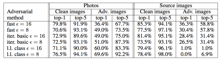
Table 1: In the average case, the accuracy of the image of the confrontational image (randomly selected image).
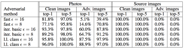
Table 2: Accuracy of photographs of confrontational images in pre-screening situations (clean images are correctly classified, and confrontational images ensure incorrect classification).

Table 3: Destruction rate of confrontational images of photographs.
3.3 Experimental Results of Antagonistic Image Photographs
The picture conversion experiment results are summarized in Tables 1, 2 and 3.
We found that "fast" confrontational images are more powerful for photo conversion than iterative methods. This can be explained by the fact that iterative methods use more subtle perturbations that are more likely to be destroyed by image transformations.
An unexpected result is that, in some cases, the rate of resistance destruction is higher in the "pre-screening situation" than in the "average situation." In the case of the iterative method, the total power of even pre-screened images is lower than that of randomly selected images. This means that to get a very high level of confidence, iterative methods often make subtle adjustments that do not adapt to image transformations.
Overall, the results show that some parts of the adversarial case are still misclassified even after a non-negligible transformation: picture transformation. This proves the possibility of physical antagonistic examples. For example, an adversarial example using the fast method of ε = 16 can predict that 2/3 of the images will appear in the previous misclassification and 1/3 of the images will appear in the top 5 misclassification. Therefore, by generating enough confrontational images, the anticipation of resistance may cause far more misclassification than natural input.
4, artificial image conversion
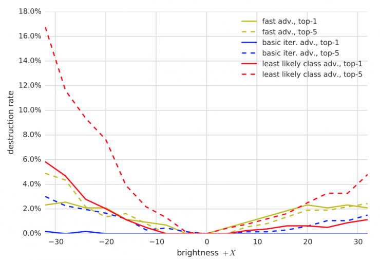
Figure 5: Comparison of the rate of conquering and destroying of various methods of confrontation to change the brightness. All experiments were performed with ε = 16 .
The picture transformation described in the previous section can be considered as a more simple synthesis of image transformation. Therefore, in order to better understand, we conducted a series of experiments to measure the rate of destructive destruction of artificial images. We explored the following conversion groups: changing contrast and brightness, Gaussian blur, Gaussian noise, and JPEG encoding.
For this set of experiments, we used a subset of 1,000 images and randomly selected them from the validation set. The 1,000 subsets are selected once, so that all experiments in this section use the same subset of images. We experimented with multiple pairs of antagonistic methods and transformations. For each set of transformation and antagonistic methods, we calculate the antagonistic examples, apply transformations to the antagonistic examples, and then calculate the destruction rate according to equation (1).
When ε = 16, the results of various transformation and antagonistic methods are summarized in Figures 5, 6, 7, 8 and 9. We can draw the following general observations:
The counterexamples generated by the quick method are the strongest in terms of conversions, and the least likely type of methods generated by the iteration is the weakest. This is consistent with our results in the image conversion.
The first five damage rates are usually higher than the first one. This can be interpreted as: In order to “destroy†the first five examples of confrontation, there must be a transformation to advance the correctly classified label into one of the top five predictions. However, in order to destroy the former antagonistic example, we must push the correct label into the first prediction, which is a more stringent requirement.
Changing the brightness and contrast does not have much effect on the antagonistic example. The destruction rate of the fast method and the basic iterative anti-cone case is less than 5%, and the failure rate of the iterative least likely category method is less than 20%.
Blurring, noise, and JPEG encoding have a higher rate of corruption than changing the brightness and contrast. Especially for iterative methods, the destruction rate can be as high as 80% - 90%. However, none of the conversions destroyed 100% of the antagonistic examples, which is consistent with the results in the "image transformation" experiment.

Fig. 6: Comparison of the resistance destruction rates of various antagonistic methods for changing the contrast. All experiments were performed with ε = 16 .
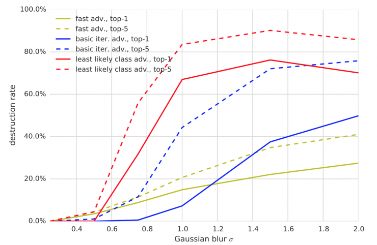
Figure 7: Comparison of the percentage of conquering and destruction of various methods of confrontation of Gaussian fuzzy transformation. All experiments were performed with ε = 16 .
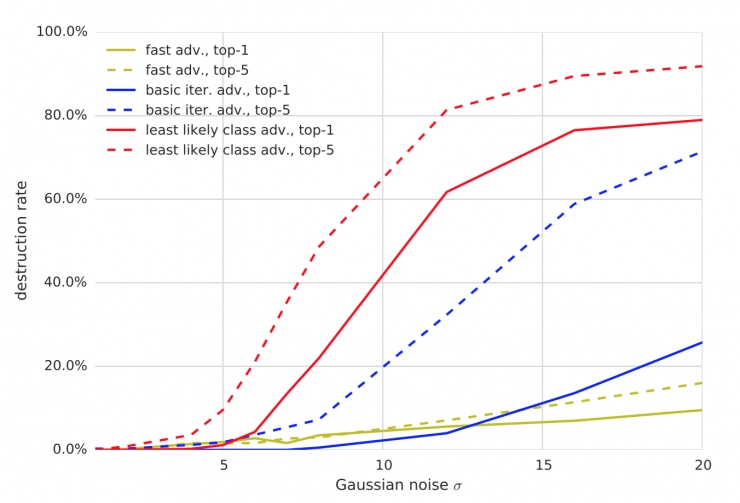
Figure 8: Comparison of the rate of concomitant destruction of various antagonistic methods of Gaussian noise transformation. All experiments were performed with ε = 16 .
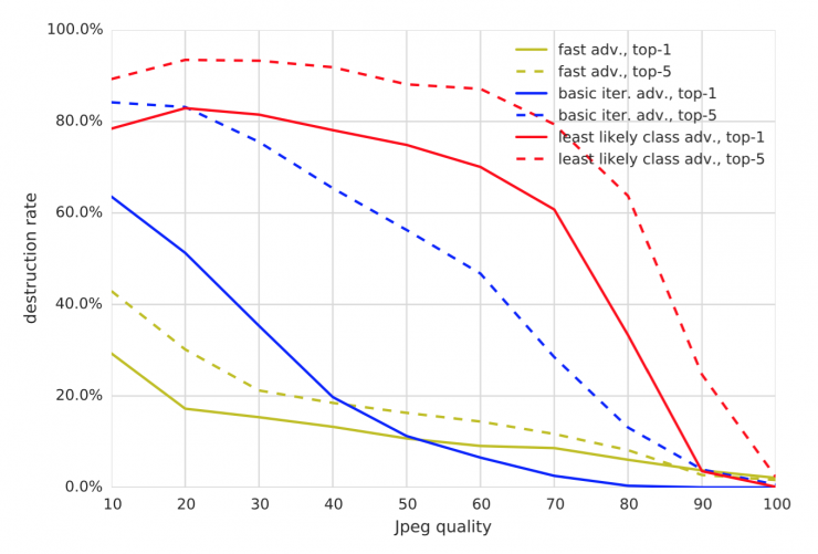
Figure 9: Comparison of the percentage of conquering and destroying of various methods of antagonism of JPEG code transformation. All experiments were performed with ε = 16 .
5 Conclusion
In this paper, we explored the possibility of creating adversarial examples for machine learning systems that operate in the physical world. We used an image taken with a cell phone camera and entered an Inception v3 image classification neural network. We have shown that in such a setting, there are enough parts in the confrontational image made using the original network to be misclassified, even if the classifier is input by the camera. This discovery proves the possibility of a hostile example of a machine system in the physical world. In future research, we expect to prove that it is also possible to use other types of physical objects besides images printed on paper to attack different types of machine learning systems—such as complex reinforcement learning agents—without involving parameters of the model and The architecture can implement attacks (assuming the use of the transfer feature), as well as by explicitly simulating physical transformations in the process of building counterexamples, thereby realizing higher success rate physical attacks. We also hope that future research will develop effective methods to defend against such attacks.
Via MIT Tech Review